Evaluating a particle size distribution

In general, most particle size distributions that I measured during my career have been best fit by a lognormal distribution. Sometimes one encounters a specimen that is better described by a normal (Gaussian) distribution. It is important to have tools that permit the analyst to scrutinize the results.

In this case our specimen was a dispersion of silver halide particles. These were imaged at -170C in a cooling holder to minimize radiolysis (mass loss of the halide and reduction to Ag⁰). This is a useful data set, so I included the measurements in my rAnaLab R package.

A representative field is shown below:

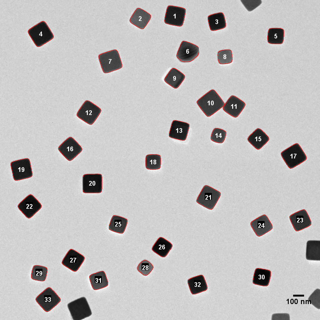
Figure 1: An image of well-dispersed AgX grains imaged at -170C.

We can first compare the parametric statistics from both distributions. The rAnaLab package has a function that makes this convenient.

library(rAnaLab)
data(diam)

ret <- calc.normal.lognormal.stats(diam$ecd.nm)
pander::pander(ret)

nobs	mu	s	geom mean	geom sd
2123	131.4	17.07	130.2	1.141

Note that the mean value of the two distributions agree within about 1.5 nm. Let’s next look at a panel plot comparing the data to a normal distribution.

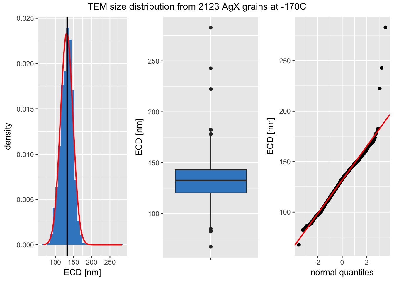
An panel plot from well-dispersed AgX grains imaged at -170C. **Left:** Histogram and Kernel Density plot. **Center:** A boxplot highlighting outliers. **Right** A plot comparing the measured values to a Normal distribution.

Figure 2: An panel plot from well-dispersed AgX grains imaged at -170C. Left: Histogram and Kernel Density plot. Center: A boxplot highlighting outliers. Right A plot comparing the measured values to a Normal distribution.

I find the panel plot particularly helpful. We only see deviations from the Normal distribution at the extreme tails.

We can now compare to a single mode lognormal distribution. We will first bin the data with a spacing of the 8^th root of 2. Again, this has been encapsulated into two function calls. Finally, we will plot the data


l.b <- rb.lognormal.bin(diam[,1], n.root.2=8.0,  base.val=10.0)
binned <- make.log.bin.df(l.b)
plt <- ggp.logx.distn(binned,
                      "AgX Lognormal Grain Diameter",
                       x.units=-9,
                       d.max=0.025,
                       limits=c(50, 500),
                       breaks=c(50, 100, 500),
                       minor_breaks=c( 60, 70, 80, 90, 200, 300, 400))

print(plt)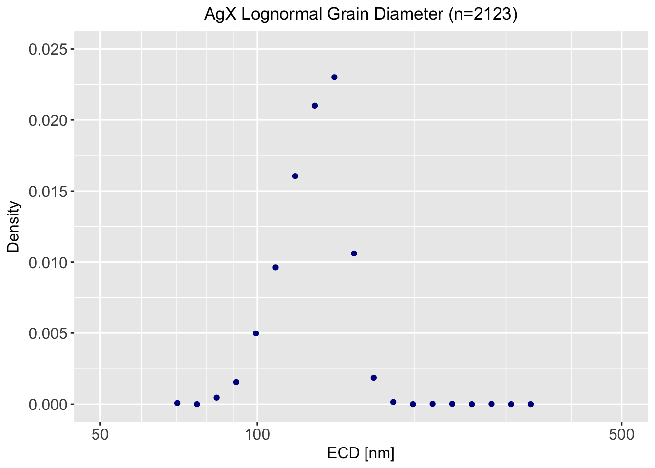

We don’t gain anything in this case by going to a lognormal distribution and it appears slightly skewed. We will follow Occam’s Razor (loosely translates, “It is vain to do with more what can be done with fewer”).

Characterizing a Particle Size Distribution

Evaluating a particle size distribution